Variational Inference

June 2017 - Alberto Pou

In this post, I’ll be discussing probabilistic machine learning. Over the past months, I’ve been learning about this field, specifically a type of inference known as Variational Inference, which was the topic of my master’s thesis. I’d like to share a summary of my experience.

Probabilistic Machine Learning

Recent decades of machine learning research have produced a wide variety of algorithms covering areas such as autonomous vehicles, medical diagnosis, speech recognition, and user ranking for marketing campaigns. These algorithms are primarily based on constructing a model that describes data as closely as possible.

A model is a compact description of a dataset that enables predictions about future samples. The key difference between conventional machine learning models and probabilistic ones is that the latter can model uncertainty. In other words, they tell us how likely a prediction is to be correct. This is particularly valuable in fields like medicine or finance, where making a wrong decision could harm someone’s health or lead to financial losses.

Probabilistic models use probability theory to incorporate prior information, so the algorithm isn’t based solely on sample data. They permit the use of different datasets for learning (useful when data is scarce) and allow defining complex models with any number of required random variables. They also support online learning, where you do not need to retrain the entire model when you obtain new data; you simply update some probabilities. They are particularly useful in decision-making scenarios where a robust explanation of the model is required. Finally, as generative models, they can generate new data by sampling from the inferred distributions.

Unlike discriminant models that only model the probability of the target variable, generative models are complete models that use all variables (observed and latent), allowing multiple questions to be answered.

The construction of these models with latent variables follows the Box Loop philosophy, created by statistician George E. P. Box. This loop is iterated several times during model construction:

1. First, a probabilistic model is built based on existing domain knowledge
2. Patterns are discovered using the model and an inference method
3. Finally, the model is validated. If it’s not good enough, we return to step 1

Bayesian Inference

Bayesian inference attempts to reveal hidden structure in data that cannot be directly observed. In traditional machine learning, parameters are values determined by optimization algorithms that minimize an error function. The Bayesian perspective is different: all unknown parameters are described by probability distributions, and observing evidence allows us to update these distributions using Bayes’ rule.

Bayes’ Rule

Bayes’ rule describes how a prior probability about an event should be updated after observing evidence. From a Bayesian perspective, there is no distinction between parameters and observed variables, as both are random variables. We use x for observed variables and θ for latent variables.

$p(\theta|x) = \frac{p(x|\theta)p(\theta)}{p(x)}$

The formula components are:

• Posterior p(θ|x): The probability of parameters given the data, defined as the probability that the model with parameters θ generated data x
• Likelihood p(x|θ): The probability of data assuming a parameterized distribution, commonly used to assess model quality
• Prior p(θ): The probability of parameters before observing data, reflecting our prior knowledge
• Evidence p(x): Calculated as ∫p(x,θ)dθ. While often intractable to compute, it’s a normalizing constant and doesn’t affect comparisons between models on the same data

Using likelihood to estimate θ is called Maximum Likelihood Estimation (MLE), while including the prior gives Maximum A Posteriori estimation (MAP). MLE and MAP are equivalent with a uniform prior. However, these methods only estimate a mean, median, or mode of the posterior. If you need to model uncertainty or generate new data, you need the full posterior distribution. Methods like Variational Inference (VI) or Markov Chain Monte Carlo (MCMC) allow inferring this distribution.

A simple example: Initially, we believe (prior) that the height of Barcelona’s population follows a Normal distribution. After observing sample heights (evidence), our belief about this distribution must be updated. The posterior distribution reflects this updated belief.

It’s an iterative process: the posterior from one iteration becomes the prior for the next.

Posterior Approximation

Probabilistic machine learning uses latent variables to describe hidden data structure. Inference algorithms estimate the posterior, which is the conditional distribution of latent variables given observed variables. Since we typically work in high-dimensional spaces, computing the posterior expectation is often impossible analytically and computationally. Two main algorithmic approaches have emerged:

• Markov Chain Monte Carlo (MCMC): Sampling-based approximate inference. It builds a Markov chain over latent variables where the posterior is the stationary distribution. Known algorithms include Metropolis-Hastings, Gibbs sampling, and Hamiltonian Monte Carlo.

• Variational Inference (VI): Optimization-based approximate inference. It creates an analytical approximation (the variational model) that’s adjusted to minimize distance from the posterior.

Probabilistic Graphical Models

In Bayesian statistics, a model represents a joint probability over all random variables.

$p(x_1, \ldots, x_n, \theta_1, \ldots, \theta_m)$

Probabilistic graphical models provide a practical way to represent these models. They’re directed graphs where nodes are random variables and edges represent dependency relationships. Plates (rectangles with a count) denote vectors of random variables.

Local and Global Variables

Probabilistic models distinguish between global variables (shared across all data points) and local variables (specific to each data point). Shaded nodes represent observed variables.

Variational Inference

Strategy

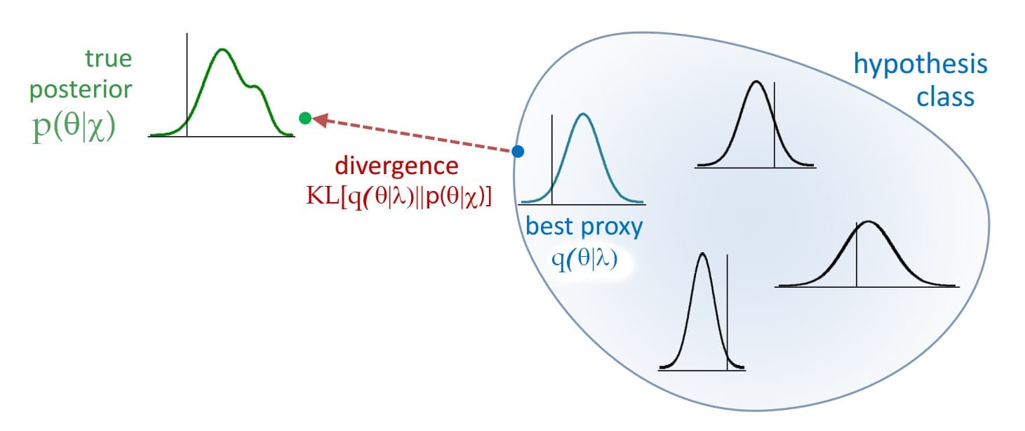
Variational Inference defines a distribution q(θ|λ) whose parameters λ are optimized to reduce the distance from the posterior p(θ|x). This new distribution is the variational model, and the posterior is the probabilistic model. The goal is to optimize λ to minimize the divergence between them.

Kullback-Leibler Divergence

Euclidean distance between distribution parameters is an imperfect similarity measure since we are comparing distributions, not points. Consider N(0, 5) and N(5, 5); they are quite similar despite being 5 units apart. Compare this to N(0, 5) and N(2, 7), which seem more different but have Euclidean distance of only 4.

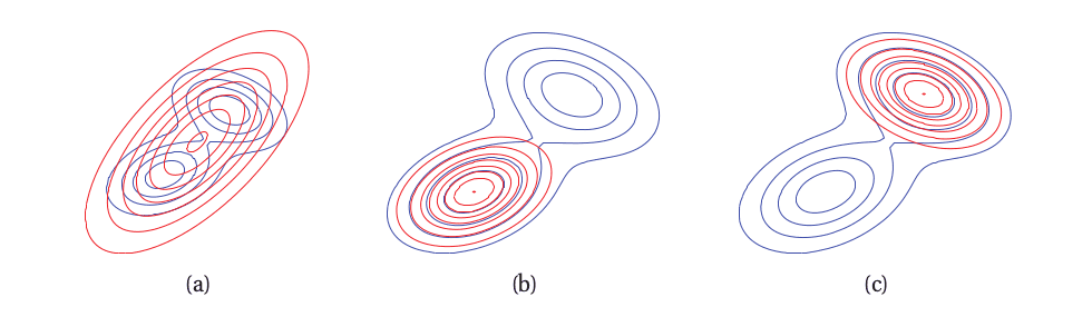
We use Kullback-Leibler divergence (KL), which quantifies information loss when approximating one distribution with another. KL is asymmetric: KL[p||q] ≠ KL[q||p]. Forward KL is used in Expectation Propagation, while VI uses reverse KL.

$H = -\sum_{i=1}^{N} p(x_i) \ln p(x_i)$

$KL[q(\theta|\lambda)||p(\theta|x)] = \int q(x_i)(\ln q(x_i) - \ln p(x_i))$

$KL[q(\theta|\lambda)||p(\theta|x)] = \int q(\theta|\lambda) \ln \frac{q(\theta|\lambda)}{p(\theta|x)}$

The visualization below compares forward and reverse KL when approximating a bimodal distribution:

Mean-Field Assumption

$q(\theta|\lambda) = \prod_i q_i(\theta_i|\lambda_i)$

The Evidence Lower Bound (ELBO)

Finding the best posterior approximation requires minimizing the Kullback-Leibler divergence (KL) between the variational model q(θ|λ) and the probabilistic model p(θ|x).

Starting from Bayes’ rule, we can derive:

$p(\theta|x) = \frac{p(x|\theta)p(\theta)}{p(x)} \Rightarrow p(x) = \frac{p(x,\theta)}{p(\theta|x)} \Rightarrow$

$\ln p(x) = \ln \frac{p(x,\theta)}{p(\theta|x)} \Rightarrow \int q(\theta|\lambda) \ln \frac{p(x,\theta)}{p(\theta|x)} d\theta \Rightarrow$

$\int q(\theta|\lambda) \ln \frac{p(x,\theta)}{p(\theta|x)} \frac{q(\theta|\lambda)}{q(\theta|\lambda)} d\theta \Rightarrow \int q(\theta|\lambda) \left( \ln \frac{q(\theta|\lambda)}{p(\theta|x)} + \ln \frac{p(x,\theta)}{q(\theta|\lambda)} \right) d\theta \Rightarrow$

$\ln p(x) = \int q(\theta|\lambda) \ln \frac{q(\theta|\lambda)}{p(\theta|x)} d\theta + \int q(\theta|\lambda) \ln \frac{p(x,\theta)}{q(\theta|\lambda)} d\theta$

This expression gives us a more tractable way to work with the model evidence:

• $\int q(\theta|\lambda) \ln \frac{q(\theta|\lambda)}{p(\theta|x)} d\theta$: $KL[q(\theta|\lambda)||p(\theta|x)]$
• $\int q(\theta|\lambda) \ln \frac{p(x,\theta)}{q(\theta|\lambda)} d\theta$: Model Evidence Lower Bound ($ELBO(q(\theta|\lambda), p(x, \theta))$)

$\boxed{\ln p(x) = KL[q(\theta|\lambda)||p(\theta|x)] + ELBO(q(\theta|\lambda), p(x, \theta))}$

This derivation shows that minimizing KL[q(θ|λ)||p(θ|x)] is equivalent to maximizing ELBO(q(θ|λ), p(x,θ)), which is much easier to evaluate. An intractable integral has been transformed into an expectation over a known distribution.

Variational Inference uses ELBO as the stopping criterion. When the ELBO value stops increasing across iterations, we’ve found good values for the variational parameters λ that bring us close to the probabilistic model (the posterior).

We can rewrite ELBO as:

$ELBO(q(\theta|\lambda), p(x, \theta)) = \int q(\theta|\lambda) \ln \frac{p(x,\theta)}{q(\theta|\lambda)} d\theta$

$= \int q(\theta|\lambda) \ln p(x, \theta) d\theta - \int q(\theta|\lambda) \ln q(\theta|\lambda) d\theta$

$= \mathbb{E}_{q(\theta|\lambda)}(\ln p(x, \theta)) - \mathbb{E}_{q(\theta|\lambda)}(\ln q(\theta|\lambda))$

Where each term represents:

• $\mathbb{E}_{q(\theta)}(\ln p(x, \theta))$: Expectation of the joint probability of the probabilistic model
• $\mathbb{E}_{q(\theta)}(\ln q(\theta|\lambda))$: Shannon entropy

Applying the Mean-Field assumption, ELBO becomes:

$ELBO(q(\theta|\lambda), p(x, \theta)) = \int q(\theta|\lambda) \ln \frac{p(x,\theta)}{q(\theta|\lambda)} d\theta$

$= \int \prod_i q_i(\theta_i|\lambda_i) \left( \ln p(x, \theta) - \sum_i \ln q_i(\theta_i|\lambda_i) \right) d\theta$

Variational Inference Algorithm

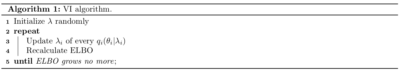
This algorithm represents the basic idea of VI. In practice, several additional considerations are necessary. First, the variational model may contain both local and global variables that must be updated in specific ways. You also need to choose an inference method: Coordinate Ascent, Gradient Ascent, or Stochastic Gradient Descent. The choice does not change the basic VI structure; it only affects how the λ parameters are updated in each iteration.

Coordinate Ascent Variational Inference

The most traditional method is Coordinate Ascent Variational Inference (CAVI). Implementing CAVI requires knowledge of Bayesian statistics because updating each variational parameter λ requires deriving analytical closed-form expressions.

When the model is completely conjugate (like Dirichlet-Categorical or Normal-Inverse-Wishart-Normal), the posterior can be calculated analytically without approximation. However, with vast amounts of data, these analytical calculations become impractical due to large matrix operations. In such cases, and for non-conjugate models, approximating the posterior using VI is a good option.

The analytical updates for variational parameters can be derived two ways: generic derivation or using properties of the Exponential Family.

Generic derivation uses the following formula (assuming Mean-Field):

$q(\theta_i|\lambda_i) \propto exp(\mathbb{E}_{q(\theta_{\neq i}|\lambda_{\neq i})}[ln(p(x, \theta))])$

This derivation must be done for each variable θ_i. A statistician can then deduce the distribution type and update rule for each variational parameter.

Alternatively, updates can be derived using Exponential Family properties. This family includes all distributions expressible as:

$p(x|\theta) = h(x) exp(\eta(\theta) t(x) - a(\eta(\theta)))$

Where:

• h(x): Base measure
• η(θ): Natural parameters (depends only on parameters)
• t(x): Sufficient statistics (depends only on data)
• a(η(θ)): Cumulant (normalizer)

This family enables conjugacy relationships between distributions, when the joint distribution simplifies nicely, allowing analytical posterior calculation.

CAVI Algorithm

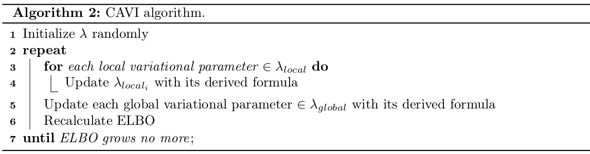
This CAVI version already distinguishes between updating local and global variables.

Gradient Ascent Variational Inference

A more straightforward alternative is Gradient Ascent Variational Inference (GAVI). Instead of analytically deriving update formulas, it uses an exploratory optimization process based on Gradient Ascent.

Gradient Ascent

$\lambda = \lambda - \eta \nabla_\lambda \mathbb{C}(\lambda)$

Recent years have seen optimizations like Momentum, Adagrad, Adadelta, RMSprop, and Adam. These improvements include per-parameter learning rates and using gradient history to inform updates.

GAVI Algorithm

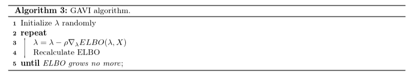
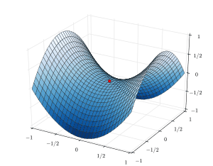
A problem with using the gradient is that it assumes the latent variable space is Euclidean, implying distances between distributions are measured by Euclidean distance of their parameters. The solution is the natural gradient, which accounts for the true distance between distributions.

$\hat{\nabla}_\lambda \mathbb{C}(\lambda) \approx \mathbb{G}(\lambda)^{-1} \nabla_\lambda \mathbb{C}(\lambda)$

The natural gradient indicates the direction of maximum slope in Riemannian space, where the true distance between distributions is considered. This is computed by pre-multiplying the standard gradient by the inverse of Fisher’s information matrix G(λ).

$\mathbb{G}(\lambda) = \mathbb{E}_\lambda[(\nabla_\lambda ln(q(\theta|\lambda)))(\nabla_\lambda ln(q(\theta|\lambda)))^T]$

CAVI’s analytical updates already account for distribution shapes when measuring distances.

Efficiency Problems

In the information age, machine learning algorithms process massive datasets. This requires scaling algorithms or designing less computationally expensive alternatives. CAVI and GAVI must pass through all data in each iteration, which becomes intractable for massive datasets.

Stochastic Variational Inference

The solution is Stochastic Variational Inference, which uses a batch (subset) of data in each iteration. While requiring more iterations than conventional approaches, it converges to a local optimum without keeping the entire dataset in memory.

Stochastic Optimization

This technique obtains estimates of the true gradient using data subsets. The algorithm iterates over batches and adjusts the model’s hidden structure based only on that batch.

$\lambda = \lambda - \rho \nabla_\lambda \mathbb{C}(\lambda, x)$

The expectation of the estimated gradient $\mathbb{E}(\nabla_\lambda \mathbb{C}(\lambda, x))$ using a batch $x$ equals the true gradient $\nabla_\lambda \mathbb{C}(\lambda, X)$ over the full dataset $X$.

Under ideal conditions, stochastic algorithms converge to a local optimum if the learning rate ρ satisfies the Robbins-Monro conditions:

This technique yields Stochastic Gradient Ascent Variational Inference (SGAVI) or Stochastic Natural Gradient Ascent Variational Inference (SNGAVI) when using natural gradients. These algorithms can avoid saddle points thanks to gradient estimation noise.

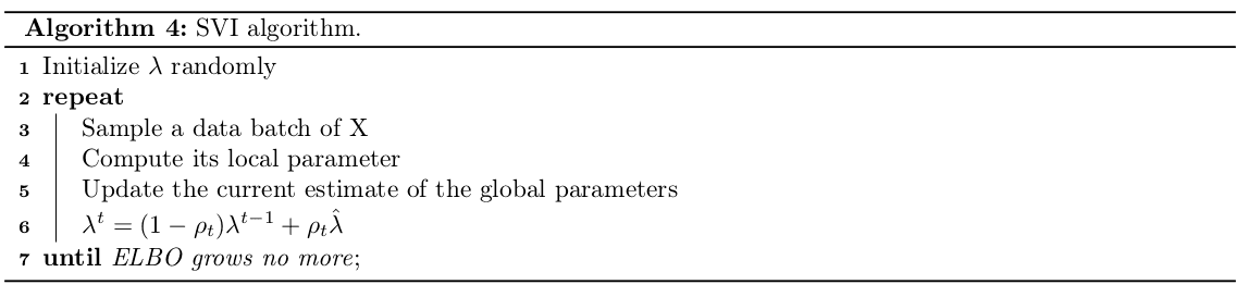
Algorithm

When updating variational parameters via closed analytical formulas, the algorithm is Stochastic Coordinate Ascent Variational Inference (SCAVI). When using stochastic optimization, it’s SGAVI. The stochastic version uses a correction term incorporating calculations from previous iterations:

Black Box Variational Inference

Starting from the ELBO formula derived earlier:

$ELBO(q(\theta|\lambda), p(x, \theta)) = \mathbb{E}_{q(\theta|\lambda)}(\ln p(x, \theta)) - \mathbb{E}_{q(\theta|\lambda)}(\ln q(\theta|\lambda))$

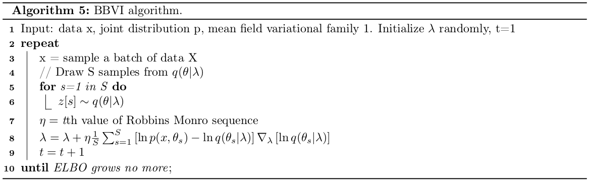
Black Box Variational Inference (BBVI) samples from the variational model q(θ|λ) to approximate the expectations in the formula. These expectations can be computationally expensive and create memory bottlenecks.

Score Gradients

Applying gradients and algebraic transformations to the ELBO formula:

$\nabla_\lambda ELBO(q(\theta|\lambda), p(x, \theta)) = \nabla_\lambda \mathbb{E}_{q(\theta|\lambda)}(\ln p(x, \theta)) - \mathbb{E}_{q(\theta|\lambda)}(\ln q(\theta|\lambda))$

$= \int [\ln p(x, \theta) - \ln q(\theta|\lambda)] \nabla_\lambda q(\theta|\lambda) d\theta$

After these transformations, we do not need gradients of the complete ELBO; it is sufficient to differentiate only the variational model q(θ|λ).

Monte Carlo Integration

Monte Carlo integration approximates integrals by sampling the variable being integrated over and summing the function values at those samples. More samples yield more accurate approximations.

$\nabla_\lambda ELBO(q(\theta|\lambda), p(x, \theta)) \approx \frac{1}{S} \sum_{s=1}^{S} [\ln p(x, \theta_s) - \ln q(\theta_s|\lambda)] \nabla_\lambda [\ln q(\theta_s|\lambda)] \quad \text{where} \quad \theta_s \sim q(\theta|\lambda)$

Algorithm

Considerations

This algorithm results from various approximations that can affect convergence. The Mean-Field assumption and Monte Carlo integration both introduce variance, potentially causing slow convergence. Variance reduction techniques include:

• Rao-Blackwellization: Reduces variance of a random variable by replacing it with its conditional expectation over a subset of variables
• Control Variates: Replaces the Monte Carlo expectation with a lower-variance function

A major advantage is that we don’t need to derive analytical update formulas or analytical ELBO expressions. This makes these algorithms accessible to people with less statistical background (like myself). Another approach, Automatic Differentiation Variational Inference (ADVI), shares these advantages and improves convergence for non-conjugate models that challenge other VI variants.

Previously, VI could only handle conjugate models since non-conjugate models weren’t easily derivable. Algorithms like ADVI and BBVI enabled inference for these models by replacing analytical calculations with approximate strategies.

Libraries for Variational Inference

Popular libraries for VI and Markov Chain Monte Carlo (MCMC):

• Edward: Uses TensorFlow for gradient computation; implements BBVI, reparameterization BBVI, and Metropolis-Hastings
• Stan: Uses C++ automatic differentiation (reverse mode); implements ADVI and HMC
• PyMC: Uses PyTensor for gradients; implements ADVI, Gibbs sampling, and Metropolis-Hastings
• Bayesflow: Google’s module for VI in TensorFlow

For more on Variational Inference and probabilistic model inference, check out my master’s thesis. It focuses on using automatic differentiation tools to apply Variational Inference to Gaussian Mixture Models (GMM). The repository contains GMM implementations using TensorFlow, Edward, Autograd, and other technologies.

References

• Variational Inference in Gaussian Mixture Models (Alberto Pou)
• Science and Statistics (George E. P. Box)
• Build, Compute, Critique, Repeat: Data Analysis with Latent Variable Models (David M. Blei)
• Probabilistic Graphical Models: Principles and Techniques (Koller & Friedman)
• Model-Based Machine Learning (Christopher M. Bishop)
• Machine Learning: A Probabilistic Perspective (Kevin P. Murphy)
• An Overview of Gradient Descent Optimization Algorithms (Sebastian Ruder)
• Variational Bayesian Inference (Slides) (Kay H. Brodersen)
• Variational Inference: A Review for Statisticians (David M. Blei)
• Stochastic Variational Inference (Hoffman, Blei, Wang & Paisley)
• Black Box Variational Inference (Ranganath, Gerrish & Blei)
• The Stan Math Library: Reverse-Mode Automatic Differentiation in C++ (Carpenter et al.)
• Automatic Differentiation Variational Inference (Kucukelbir et al.)