Automatic Differentiation

March 2017 - Alberto Pou

Derivatives, specifically gradients (derivatives in multidimensional spaces) and Hessians (second derivatives), have become fundamental to machine learning. The gradient is a vector that indicates the direction of maximum slope of a function at a given point. This is crucial for navigating the function space to find local minima or maxima. The Hessian provides information about the concavity and convexity of the function, which some algorithms use to improve exploration and find optima faster.

Automatic Differentiation (AD) is an efficient and accurate procedure for calculating derivatives of numerical functions represented as computer programs. Model optimization, from a mathematical perspective, involves minimizing or maximizing a function, and derivatives are the essential tool for accomplishing this.

There are several methods for computing derivatives with a computer:

Numerical differentiation: This method uses the definition of the derivative to approximate values using samples of the original function. We can approximate the gradient ∇f using finite differences, where we evaluate the function at nearby points and compute the slope.

Derivative definition

Symbolic differentiation: This approach involves automatic manipulation of mathematical expressions to obtain derivatives, similar to what we learned in calculus class. It requires implementing rules of differentiation. The main drawback is that it can produce lengthy symbolic expressions that are difficult to evaluate.
Automatic Differentiation: This method is based on the fact that all functions can be decomposed into a finite number of operations whose derivatives are known. By combining these derivatives, we can compute the derivative of the original function. Applying the chain rule to each elementary operation yields the computation trace for the actual function derivative.

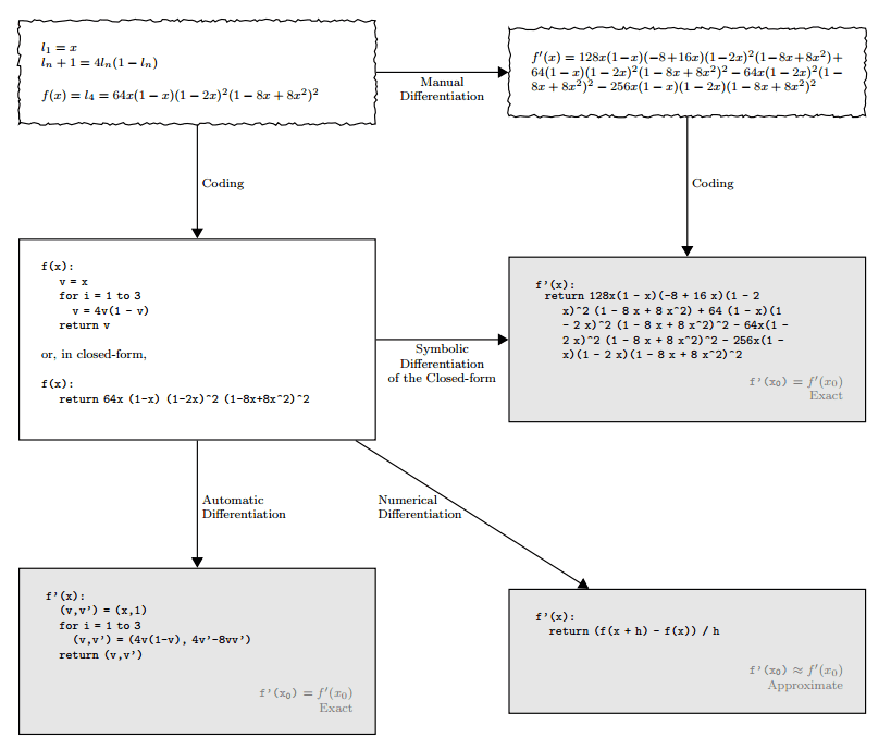
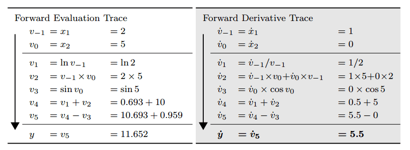
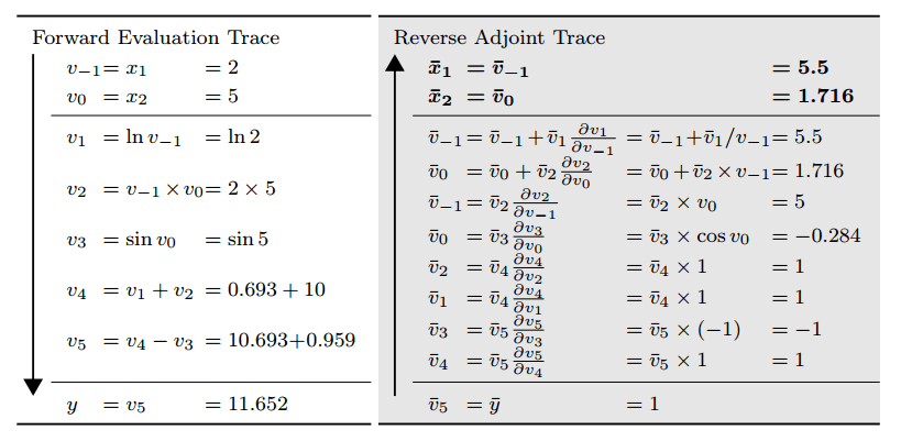
There are two modes of Automatic Differentiation: forward mode and reverse mode. Forward mode evaluates the function parts forward, then computes each part of the derivative until the final result is obtained. Reverse mode evaluates the function parts forward but then, starting from the derivative of the function, computes the partial derivatives backward.

This is exactly how backpropagation works in neural networks, where partial derivatives are needed to update the weights of each layer. This method allows reusing previously computed values and calculating derivatives very efficiently.

AD forward mode

AD reverse mode

Derivative Tools

Here are some popular software packages for computing derivatives and gradients:

TensorFlow: Uses AD reverse mode
Theano: Uses symbolic differentiation
Mathematica: Uses symbolic differentiation
Autograd: Uses AD reverse mode

TensorFlow

TensorFlow is an open source library developed by Google for numerical computation using flow graphs. Before executing a program, TensorFlow builds a flow graph where nodes represent mathematical operations and edges represent multidimensional data arrays called tensors. This graph structure allows optimal utilization of the system’s CPUs and GPUs, enabling transparent parallelization of computations.

Originally designed for deep learning, TensorFlow makes it easy to implement Deep Neural Networks (DNNs), Convolutional Neural Networks (CNNs), and Recurrent Neural Networks (RNNs). More recent versions have expanded to serve the broader machine learning community.

One of the most interesting aspects of TensorFlow is its elegant implementation of AD reverse mode. The developer defines a model with parameters as variables, specifies the inference algorithm, and TensorFlow automatically handles gradient computation and optimization.

Usage Examples

Below is the code to optimize parameters of a linear regression model with TensorFlow and Autograd (both use AD reverse mode for gradients). A linear regression model is defined by the equation:

Linear regression equation

Where w represents the weight and b the bias. AD will find values for these parameters that minimize the Mean Squared Error.

TensorFlow Implementation

In TensorFlow, parameters to be optimized are defined as variables. A cost function (Mean Squared Error) is defined based on these parameters, and the optimization algorithm (Gradient Descent) is specified. The training loop samples from the dataset and computes gradients to find the direction of steepest descent, updating the parameters until a local minimum is found.

# -*- coding: UTF-8 -*-

"""
Linear regression using Tensorflow
"""

import matplotlib.pyplot as plt
import numpy as np
import tensorflow as tf

rng = np.random

# Parameters
learning_rate = 0.01
training_epochs = 100

# Training data
train_X = np.asarray([3.3, 4.4, 5.5, 6.71, 6.93, 4.168, 9.779, 6.182, 7.59,
                      2.167, 7.042, 10.791, 5.313, 7.997, 5.654, 9.27, 3.1])
train_Y = np.asarray([1.7, 2.76, 2.09, 3.19, 1.694, 1.573, 3.366, 2.596, 2.53,
                      1.221, 2.827, 3.465, 1.65, 2.904, 2.42, 2.94, 1.3])
n_samples = train_X.shape[0]

# Graph input data
X = tf.placeholder('float')
Y = tf.placeholder('float')

# Optimizable parameters with random initialization
weight = tf.Variable(rng.randn(), name='weight')
bias = tf.Variable(rng.randn(), name='bias')

# Linear model
predictions = (X * weight) + bias

# Loss function: Mean Squared Error
loss = tf.reduce_sum(tf.pow(predictions-Y, 2))/(2*n_samples)

# Gradient descent optimizer
optimizer = tf.train.GradientDescentOptimizer(learning_rate).minimize(loss)

# Initializing the variables
init = tf.global_variables_initializer()

# Launch the graph
with tf.Session() as sess:
    sess.run(init)
    for epoch in range(training_epochs):
        for (x, y) in zip(train_X, train_Y):
            sess.run(optimizer, feed_dict={X: x, Y: y})
    train_error = sess.run(loss, feed_dict={X: train_X, Y: train_Y})
    print('Train error={}'.format(train_error))

    # Test error
    test_X = np.asarray([6.83, 4.668, 8.9, 7.91, 5.7, 8.7, 3.1, 2.1])
    test_Y = np.asarray([1.84, 2.273, 3.2, 2.831, 2.92, 3.24, 1.35, 1.03])
    test_error = sess.run(
        tf.reduce_sum(tf.pow(predictions - Y, 2)) / (2 * test_X.shape[0]),
        feed_dict={X: test_X, Y: test_Y})
    print('Test error={}'.format(test_error))

    print('Weight={} Bias={}'.format(sess.run(weight), sess.run(bias)))

    # Graphic display
    plt.plot(train_X, train_Y, 'ro', label='Original data')
    plt.plot(train_X, sess.run(weight) * train_X
             + sess.run(bias), label='Fitted line')
    plt.legend()
    plt.show()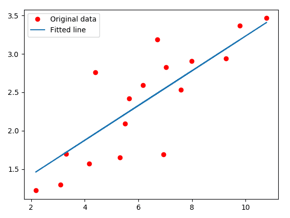

TensorFlow results

Autograd Implementation

With Autograd, the process is more explicit. We define a cost function with model parameters and then compute gradients in each iteration to update the weights.

# -*- coding: UTF-8 -*-

"""
Linear regression using Autograd
"""

import autograd.numpy as np
import matplotlib.pyplot as plt
from autograd import elementwise_grad

rng = np.random

# Parameters
learning_rate = 0.01
training_epochs = 100

# Training data
train_X = np.array([3.3, 4.4, 5.5, 6.71, 6.93, 4.168, 9.779, 6.182, 7.59,
                    2.167, 7.042, 10.791, 5.313, 7.997, 5.654, 9.27, 3.1])
train_Y = np.array([1.7, 2.76, 2.09, 3.19, 1.694, 1.573, 3.366, 2.596, 2.53,
                    1.221, 2.827, 3.465, 1.65, 2.904, 2.42, 2.94, 1.3])
n_samples = train_X.shape[0]


def loss(params):
    """ Loss function: Mean Squared Error """
    weight, bias = params
    predictions = (train_X * weight) + bias
    return np.sum(np.power(predictions - train_Y, 2) / (2 * n_samples))

# Function that returns gradients of loss function
gradient_fun = elementwise_grad(loss)

# Optimizable parameters with random initialization
weight = rng.randn()
bias = rng.randn()

for epoch in range(training_epochs):
    gradients = gradient_fun((weight, bias))
    weight -= gradients[0] * learning_rate
    bias -= gradients[1] * learning_rate
print('Train error={}'.format(loss((weight, bias))))

# Test error
test_X = np.array([6.83, 4.668, 8.9, 7.91, 5.7, 8.7, 3.1, 2.1])
test_Y = np.array([1.84, 2.273, 3.2, 2.831, 2.92, 3.24, 1.35, 1.03])
predictions = (test_X * weight) + bias
print('Test error={}'.format(
    np.sum(np.power(predictions - test_Y, 2) / (2 * n_samples))))

print('Weight={} Bias={}'.format(weight, bias))

# Graphic display
plt.plot(train_X, train_Y, 'ro', label='Original data')
plt.plot(train_X, weight * train_X + bias, label='Fitted line')
plt.legend()
plt.show()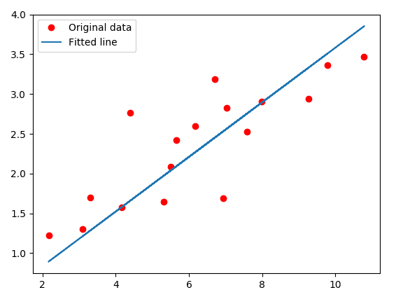

Autograd results

The main goal of this post was to shed some light on the black box of model optimization in tools like TensorFlow, Theano, and PyTorch.

References

Automatic differentiation in machine learning: a survey by Atilim Gunes Baydin, Barak A. Pearlmutter, Alexey Andreyevich Radul, Jeffrey Mark Siskind